2.1. Convolutional Neural Network (CNN) Model Theory (Basic) - Convolution, Pooling, and ReLU Function

2.1.1. Computational Cost Problem

The original motivation for introducing MLPs was to solve the problem of excessive computation in logistic regression.

Take handwritten digit recognition as an example. For a 28×28 image:

A logistic regression model with a cubic polynomial decision boundary has 80,931,145 trainable parameters
An MLP model with 784 input features, two hidden layers with 394 hidden neurons each, and 10 output neurons has 465,706 trainable parameters

But this is only a very small grayscale image. If we use an RGB image with both width and height above 100 pixels in daily life, such as 500×400, for binary classification, we would need 78,558,378 trainable parameters. That is still far too much computation.

So is there a more computationally efficient way? That is where convolutional neural networks come in.

2.1.2. Image Convolution

Think about what a computer mainly looks at when performing object recognition: contours, right? MLPs are computationally expensive because there are too many contours in the image for the computer to process. If we can first extract the main contours in the image, that is, the most critical information, and then let the MLP analyze them, we can greatly reduce the computational burden.

The step of extracting the main information requires image convolution. Image convolution refers to multiplying corresponding elements of an image matrix and a filter matrix, then summing the result to form a new matrix. Its main purpose is to quickly locate certain edge features in an image.

Mathematically, the convolution of A and B is usually written as: $$ A \ast B $$ or: $$ convolution(A, B) $$

Let us look at an example:

We have a 7×7 two-dimensional array representing an image: $$ A =

\begin{bmatrix}

X_{11} & X_{12} & X_{13} & X_{14} & X_{15} & X_{16} & X_{17} \

X_{21} & X_{22} & X_{23} & X_{24} & X_{25} & X_{26} & X_{27} \

X_{31} & X_{32} & X_{33} & X_{34} & X_{35} & X_{36} & X_{37} \

X_{41} & X_{42} & X_{43} & X_{44} & X_{45} & X_{46} & X_{47} \

X_{51} & X_{52} & X_{53} & X_{54} & X_{55} & X_{56} & X_{57} \

X_{61} & X_{62} & X_{63} & X_{64} & X_{65} & X_{66} & X_{67} \

X_{71} & X_{72} & X_{73} & X_{74} & X_{75} & X_{76} & X_{77}

\end{bmatrix} $$

We also have a 3×3 filter: $$ F =

\begin{bmatrix}

W_{11} & W_{12} & W_{13} \

W_{21} & W_{22} & W_{23} \

W_{31} & W_{32} & W_{33}

\end{bmatrix} $$ Performing the $A \ast B$ operation looks like this (this figure uses image padding, but here we will treat it as the original 7×7 size; we will talk about padding in the next article (2.2. Convolutional Neural Network (CNN) Model Theory (Advanced) - Image Padding, LeNet, and AlexNet)):

Convolution

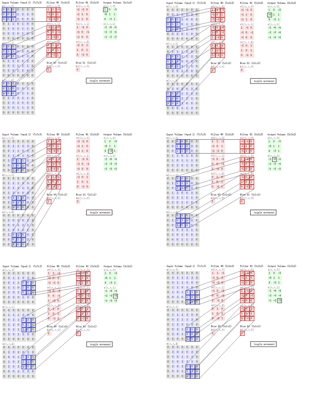
The filter is like a mask covering the image. Wherever it covers, convolution is performed there, moving pixel by pixel.

Suppose the filter is now in the upper-left corner of the image and covers: $$ \begin{bmatrix}

X_{11} & X_{12} & X_{13} \ X_{21} & X_{22} & X_{23} \ X_{31} & X_{32} & X_{33} \

\end{bmatrix} $$ Then the convolution operation performed there, multiplying and summing, is: $$ Y_{11} = X_{11} W_{11} + X_{12} W_{12} + X_{13} W_{13} + X_{21} W_{21} + X_{22} W_{22} + X_{23} W_{23} + X_{31} W_{31} + X_{32} W_{32} + X_{33} W_{33} $$

If we convolve the entire matrix, we will get a smaller matrix, from 7×7 down to 5×5: $$ Y = \begin{bmatrix} Y_{11} & Y_{12} & Y_{13} & Y_{14} & Y_{15} \ Y_{21} & Y_{22} & Y_{23} & Y_{24} & Y_{25} \ Y_{31} & Y_{32} & Y_{33} & Y_{34} & Y_{35} \ Y_{41} & Y_{42} & Y_{43} & Y_{44} & Y_{45} \ Y_{51} & Y_{52} & Y_{53} & Y_{54} & Y_{55} \end{bmatrix} $$

2.1.3. Finding Specific Features

So how do we find a specific contour in an image?

Finding Vertical Contours

Suppose we have the following image pixel matrix and want to find its vertical contour: $$ A =

\begin{bmatrix}

20 & 20 & 20 & 0 & 0 & 0 \

20 & 20 & 20 & 0 & 0 & 0

\end{bmatrix} $$

We can change the values of the filter matrix: $$ K =

\begin{bmatrix}

1 & 0 & -1 \

1 & 0 & -1

\end{bmatrix} $$ The resulting convolution output is: $$ \begin{bmatrix}

0 & 60 & 60 & 0 \

0 & 60 & 60 & 0

\end{bmatrix} $$ The grayscale values in the area containing the vertical contour are very high, so they will be highlighted in the image.

Finding Horizontal Contours

Then how do we find horizontal contours?

Suppose we have the following image pixel matrix: $$ A =

\begin{bmatrix}

20 & 20 & 20 & 20 & 20 & 20 \

0 & 0 & 0 & 0 & 0 & 0 \

0 & 0 & 0 & 0 & 0 & 0

\end{bmatrix} $$ Just rotate the filter matrix 90 degrees clockwise: $$ K =

\begin{bmatrix}

1 & 1 & 1 \

0 & 0 & 0 \

-1 & -1 & -1

\end{bmatrix} $$ The convolution result is: $$ \begin{bmatrix}

0 & 0 & 0 & 0 \

60 & 60 & 60 & 60 \

0 & 0 & 0 & 0

\end{bmatrix} $$

2.1.4. The Core of Convolutional Neural Networks

Have you noticed? The core of using convolution to find features lies in determining the values of the filter. So how do we find suitable filter values? That is where neural networks come in.

The core idea of a convolutional neural network is that the computer automatically finds suitable contour filters based on sample images and performs contour matching on new images.

Moreover, many real-world images are RGB color images, so we may need multiple filters to extract features. For RGB images, convolution is performed separately on the R, G, and B channels and then added together.

2.1.5. Pooling Layers for Dimensionality Reduction

Pooling refers to processing an image matrix according to a fixed rule and converting it into a lower-dimensional matrix.

The two most common rules are max pooling and average pooling.

Max Pooling

Max pooling means selecting the largest value in a specified region (called the pooling window size) as the representative value for that entire region.

For example: $$ \begin{bmatrix}

10 & 1 & 3 & 5 \

2 & 9 & 8 & 1 \

3 & 2 & 2 & 1 \

5 & 7 & 3 & 6

\end{bmatrix} $$ We use a 2×2 pooling window with a stride of $(2, 2)$.

$(2, 2)$ means that after scanning one region, we move 2 units horizontally, and when moving to the next row, we move 2 units vertically

The final result is: $$ \begin{bmatrix}

10 & 8 \

7 & 6

\end{bmatrix} $$

Max pooling is beneficial because it can preserve core information.

Average Pooling

Using the same data: $$ \begin{bmatrix}

10 & 1 & 3 & 5 \

2 & 9 & 8 & 1 \

3 & 2 & 2 & 1 \

5 & 7 & 3 & 6

\end{bmatrix} $$ Average pooling computes the average of all values in the pooling region as the representative value for that region.

If we still use a 2×2 pooling window with a stride of $(2, 2)$, the result is: $$ \begin{bmatrix}

5.5 & 4.25 \

4.25 & 3

\end{bmatrix} $$

In most cases, max pooling is preferred because it preserves feature information better.

2.1.6. Convolutional Neural Network

The title of this article is convolutional neural networks, but we have not explicitly mentioned that name until now. So what exactly is a convolutional neural network?

A Convolutional Neural Network (CNN) is a model formed by connecting together the series of operations mentioned above:

Convolution
Pooling
MLP

Let us walk through the whole process with an example. Suppose I have the following data: $$ A =

\begin{bmatrix}

20 & 0 & 0 & 0 & 0 & 0 & 0 \

0 & 0 & 0 & 0 & 0 & 0 & 0 \

0 & 0 & 0 & 0 & 0 & 0 & 0

\end{bmatrix} $$

Then I want to extract the vertical contour, so I use a vertical contour filter: $$ K =

\begin{bmatrix}

1 & 0 & -1 \

1 & 0 & -1

\end{bmatrix} $$ The convolution result is (7×7 input with a 3×3 filter and no padding yields a 5×5 feature map): $$ \begin{bmatrix}

60 & 0 & 0 & 0 & 0 \

40 & 0 & 0 & 0 & 0 \

20 & 0 & 0 & 0 & 0 \

0 & 0 & 0 & 0 & 0 \

0 & 0 & 0 & 0 & 0

\end{bmatrix} $$

Then we use a 2×2 pooling window with a stride of $(2, 2)$ to perform max pooling, and the result is: $$ \begin{bmatrix}

60 & 0 \

20 & 0

\end{bmatrix} $$ Finally, we flatten the two-dimensional array into a one-dimensional array and then build the MLP model as needed. You can see that the bottom layer still relies on an MLP; there is just more data preprocessing and dimensionality reduction.

Note that before pooling after convolution, we usually also apply an activation function. The activation function can:

Make some neurons output 0, helping prevent overfitting
Help the model be solved more easily

We usually choose the ReLU function as the activation function.

2.1.7. ReLU (Rectified Linear Unit) Function

The ReLU function itself is very simple: $$ f(x) = max(x, 0) $$

ReLU

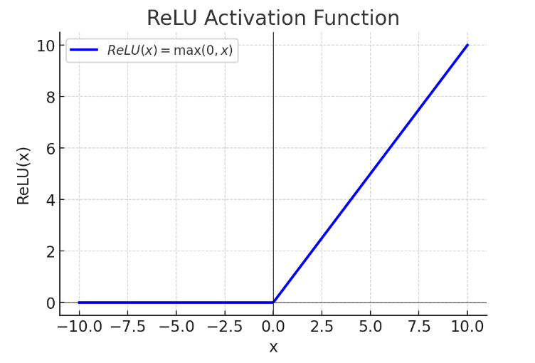
When the data is less than or equal to 0, we take 0; when it is greater than 0, we keep the original value. This behavior can:

Make the output of the convolutional layer sparser, with many values becoming 0, reducing redundant information so that the subsequent pooling layer focuses only on meaningful activations
Suppress noise and reduce interference from negative values, making the model more stable

At this point, you might ask: the logic that ReLU can perform can also be done by Sigmoid, so why not use Sigmoid? The reason is to prevent vanishing gradients: • Sigmoid: when $x \to +\infty$ or $x \to -\infty$, the gradient approaches 0, making vanishing gradients likely • ReLU: as long as $x > 0$, the gradient is 1, which keeps gradients flowing

2.1.8. Two Major Characteristics of Convolutional Neural Networks

Parameter sharing: the same feature filter can be applied to the entire image
Sparsity of connections: each node in the generated feature map is connected only to specific nodes in the original image

Keyboard shortcuts

DL Guide